

The three decades of uninterrupted economic growth and the years of fiscal surpluses are over. Australia, along with the rest of the world, faces unprecedented economic challenges that require immense budgetary responses. Stimulus spending and lower revenues in the pandemic recession have all contributed to an exponential expansion in our budget deficit and public debt (Figure 1).
Figure 1. Gross debt as a percentage of GDP
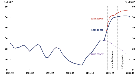 Source: Parliamentary Budget Office.
The increasing fiscal stress raises the possibility that the Australian economy might hit its maximum fiscal capacity where taxes and spending no longer adjust to stabilise debt. This stress provokes an imperative to examine the fiscal capability of Australia’s tax system to generate revenues. More specifically, there are open questions: How much additional revenue could be generated by raising taxes? What is the limit to raising taxes? Which tax has the potential to raise the most revenue? And importantly, how much debt can the government service maximally by raising taxes?
In Tran and Zakariyya (2022), we address these questions from the perspective of a long-established idea dating back to at least Arthur Laffer in the public finance literature. That is, tax revenues initially increase with the level of tax rates, reaches a maximum and then starts to decrease with further tax increases. This relationship is commonly known as the Laffer curve, stylised in Figure 2.
Figure 2. Stylised example showing fiscal space and fiscal limit
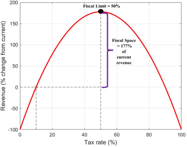
We term the maximal amount of tax revenue or tax rate at the peak of the Laffer curve as the fiscal limit. The amount of additional revenue that can be generated at the peak relative to current total revenue is the fiscal space. This quantifies the revenue generating potential of a given tax. That is, the maximum revenue that can be generated given the macroeconomic and fiscal context.
Quantifying the fiscal limit of Australia’s tax system
Quantifying the fiscal space and fiscal limit for Australia using empirical methods is a challenging task. We do not have real world data on all possible tax rates and resulting revenues. This is especially true for very high rates of taxation that would likely be closer to the fiscal limit. Instead, we use a structural macroeconomic model that matches the key macro-fiscal and distributional features of the Australian economy. In our framework, the level of taxes can be varied in counterfactual experiments. By conducting these experiments, we are able to map out the relationship between tax rates and tax revenues.
Starting from this benchmark model of the Australian economy, we simulate changes to three main taxes – consumption tax (GST), company income tax and personal income tax. In the case of income tax, we simulate changes to both its progressivity and average level of taxation. Each simulated tax change results in a counterfactual economy that we compare relative to our benchmark.
Table 1 displays our main results comparing the fiscal space and fiscal limits of the 3 taxes. The table highlights a number of important insights on revenue generating potential of Australia’s tax system.
Table 1. Summary results at the fiscal limits
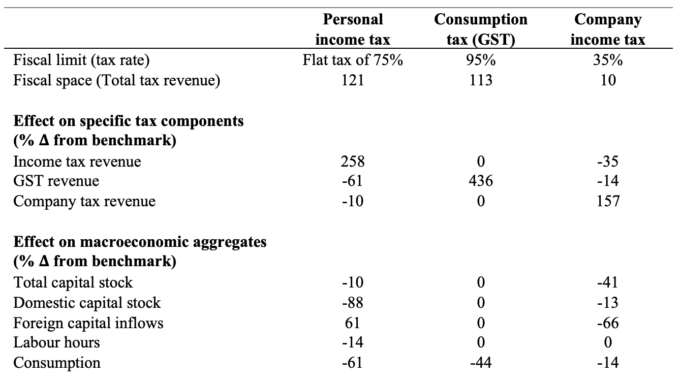
In our benchmark model economy, the greatest revenue increase is generated by a flat income tax code with a 75% tax rate. Fiscal space in terms of total revenue is 121% higher than current levels of total revenue. In contrast, there is limited scope for generating more revenue from increasing company tax rates. At its fiscal limit of 35%, total revenue generated by company tax is only 10% higher than current levels.
In our paper, we explain in detail the macroeconomic implications of increasing each of the three taxes. In what follows, we summarise some key insights that are of policy relevance at present.
Tax progressivity and income tax revenue
As Table 1 shows, income tax generates the largest fiscal space in our benchmark economy. We examine how changes in the progressive income tax code affect the maximal amount of tax revenue that the government can raise. Figure 3 illustrates the Laffer curve for income tax revenue under three alternative designs of the income tax code: (i) more progressive; (ii) less progressive; and (iii) a proportional income tax system.
Figure 3. Income tax Laffer curves at different levels of progressivity
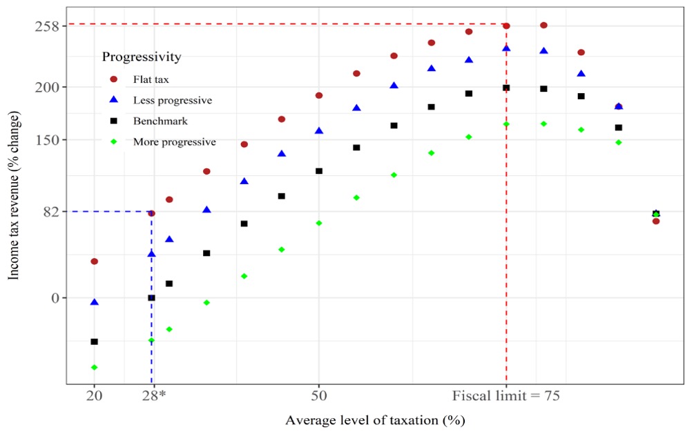
Figure 3 shows, at any given tax rate, a reduction in progressivity results in an upward shift in the Laffer curve. In this regard, if we maintain the average rate of taxation constant at benchmark levels and reduce progressivity all the way to a flat income tax, income tax revenue increases by 82%.
The rise in tax revenue with a reduction in progressivity is partly due to the fact that lower progressivity creates a positive incentive effect on labour supply. Effective marginal tax rates that rise with income discourages households from exerting extra labour effort. Flattening the tax code removes this distortion from the labour market. More importantly, in our model, lower progressivity results in a lower tax-free threshold. Coupled with the increase in labour supply this significantly increases the tax base.
The most important insight from Figure 3 is that at present, as we are nowhere near the fiscal limit for income tax, tax cuts can only worsen fiscal pressures, while tax hikes can raise more revenue.
Indirect consequences of raising one tax on other taxes
Our approach differs from empirical tax revenue forecasts in policy making. We explicitly account for intertemporal decisions of consumption, savings and work, and market price adjustments. As Table 1 reveals, these responses that affect the wider economy imply that increasing the tax rate for one tax could have indirect consequences on other tax components and in turn, total tax revenue.
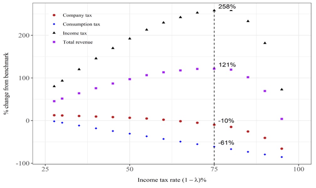
For instance, consider the case of income tax changes in Figure 4. Despite a steep rise in income tax revenue as the tax rate rises, the rise in total revenue is much smaller. This is largely due to the fact that rising income tax rates result in a decrease in revenue from the GST. In our benchmark economy, raising income tax rates lower household disposable income.
Figure 4. Effects of increasing income tax rates on the overall tax system
Sustainability of tax-financed public debt
In order to examine this, we also conduct a thought experiment where we posit that the government uses additional tax revenue to increase the stock of outstanding debt and make interest payments on it. We find that the maximum sustainable debt is attained via a flat income tax code with a 75% tax rate. Figure 5 plots the maximum sustainable debt (as a percentage of benchmark GDP) against income tax rates at varying levels of progressivity.
Figure 5. Maximum sustainable debt at various income tax rates
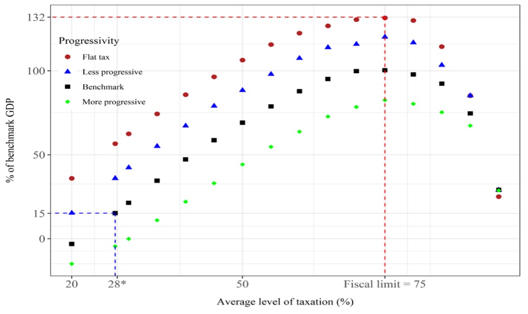
An increase in tax revenue increases the government’s ability to borrow and service more debt. As Figure 5 shows, larger public debt can be sustained with a less progressive income tax system. Currently we are nowhere near the maximum sustainable debt level of 132% of GDP.
A better understanding of fiscal limits is important in policy making
Knowing the fiscal limit provides important guidance on ways in which the government can increase revenues and its overall revenue generating potential. It also informs on the wider macroeconomic and fiscal implications of tax changes. However, there are many other subtle aspects to fully understanding fiscal limits in Australia. For example, Australia’s fiscal limit depends on policy behaviour and future fiscal surpluses/deficits, which requires an accurate depiction of the political economy.
Lack of fundamental research in policy making runs the risk of providing misleading or incomplete understandings of how unresolved fiscal stress affects the macroeconomy and how different resolutions to the growing fiscal stress will play out. This research takes initial steps to fill the void in this research area in Australia.
Other Budget Forum 2022 articles
Trusts and Tax Avoidance – Extension of Funding for ATO Taskforce, by Sonali Walpola.
Vehicle Taxing Dilemma Between Environment and Inequality, by Yogi Vidyattama, Robert Tanton and Hitomi Nakanishi.
Budget Reveals No Plan for Disaster Volunteering, by Jack McDermott.
A Fairer Tax and Welfare System for Australia, by Ben Phillips and Richard Webster.
Claiming Crypto Donations under Division 30, by Elizabeth Morton.
The Budget, Fiscal Policy and an Outbreak of Inflation, by Chris Murphy.
Natural Disasters and Government Policy Challenges, by John Freebairn.
Petrol Excise Cut in the Budget! What About the Transition to Zero-Emission Cars? by Diane Kraal.
For Social Infrastructure and Tax Reform, We Need a New Federal Fiscal Bargain, by Miranda Stewart.
A Free Lunch From Government Debt? It Certainly Looks That Way, by John Quiggin and Begoña Dominguez.


“We term the maximal amount of tax revenue or tax rate at the peak of the Laffer curve as the fiscal limit. The amount of additional revenue that can be generated at the peak relative to current total revenue is the fiscal space. This quantifies the revenue generating potential of a given tax. That is, the maximum revenue that can be generated given the macroeconomic and fiscal context.”
Your fiscal limits don’t apply in relation to empirical public finance evidence from Japan, how do you explain this?
How can fiscal limits be defined just by taxation? when taxation takes funds out of the the private sector, and reduces spending on goods and services and new investment in that sector. What are your thoughts about Modern Monetary Theory, overt monetary financing and functional finance, in relation to Public Finance?