

Why it is important to revise the Laffer Curve today? Some may argue that the Laffer Curve is an outdated concept in fiscal policy, but in the current scenario of fiscal finances, it may be useful to revisit the Laffer Curve.
There are two reasons. According to the International Monetary Fund’s Fiscal Monitor in April 2023, the level of public debt is now more elevated and projected to grow faster than foreseen before the pandemic.
In addition, most countries are revising their fiscal rules and frameworks to adapt to the post-pandemic years. Illustrative examples of this are (i) the United States’ 2024 Budget, which outlines several major tax increases for businesses and high-income individuals, (ii) the United Kingdom’s Spring Budget, which increases the corporate tax rate, and (iii) the Stage 3 tax cuts in Australia, which abolish the 37% marginal tax bracket, reduce the 32.5% marginal tax rate to 30% and raise the threshold for the 45% marginal tax rate.
In this context, the study of the revenue-raising capacity of tax systems is paramount and, therefore, revising the Laffer Curve can contribute to the debate.
What is the Laffer Curve?
The Laffer Curve is a rigorous tool often used to monitor revenue maximisation, whose origins date back to the 1970s, prompted by economist Arthur Laffer.
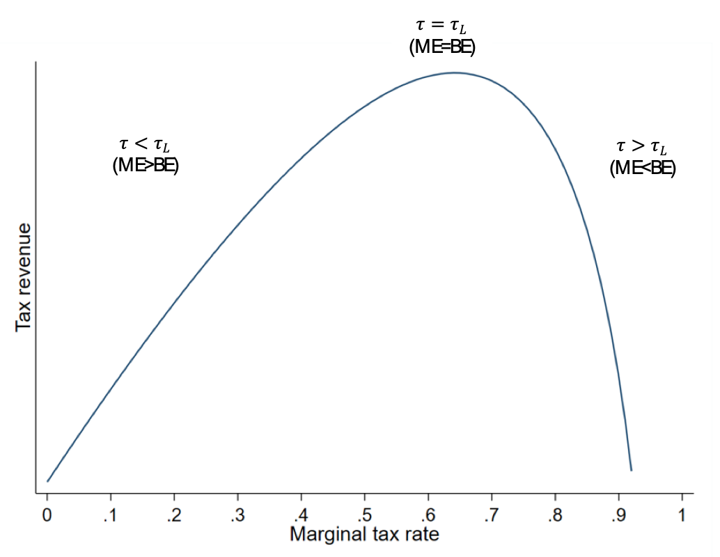
The inverted U-form of the Laffer Curve reflects the potential inverse relationship between tax rates and revenue (see Figure 1). On the ascending side of the Curve – the “normal” side – any increase in the statutory marginal tax rate (τ) raises tax revenue.
Conversely, only tax cuts can increase revenue in the descending segment – the “prohibitive” side. Thus, the peak of the Laffer Curve identifies the revenue-maximising tax rate, which represents a threshold above which any additional increase in tax rates produces a decrease in revenue.
Figure 1: Laffer Curve
 (Click to enlarge)
New development in the literature
Since the 1970s, much research has been done on the Laffer Curve, mainly from a macroeconomic perspective.
However, the literature has moved recently toward a more microeconomic-oriented analysis. In addition, more attention has also been given to modelling the complexities of current income tax structures. This tendency towards micro-oriented analysis and more detailed modelling of the tax design is due to the firm recognition that each taxpayer faces his own Laffer Curve.
Consequently, identifying the side on which each taxpayer falls within its own Laffer Curve, separately and individually, becomes the critical issue. Only after this first query is answered will it be possible to refer to the Laffer Curve of an economy or a country, which will be interpreted as the algebraic sum of all the taxpayers’ individual Laffer Curves.
Several studies have also made analytical efforts to introduce the complexities of modern personal income tax (PIT) designs into modelling the Laffer Curve. These efforts have benefited from the increased availability of tax microdata and the development of a sufficient statistic, the elasticity of taxable income (ETI).
The Laffer Curve updated
To characterise the Laffer Curve, our latest study derives analytical expressions for the revenue-maximising tax rates in the context of schedular multi-rate income taxes with income shifting. These analytical expressions are computed for the individual taxpayer and the aggregate population.
In the characterisation of the individual Laffer Curve, there are many relevant factors to consider.
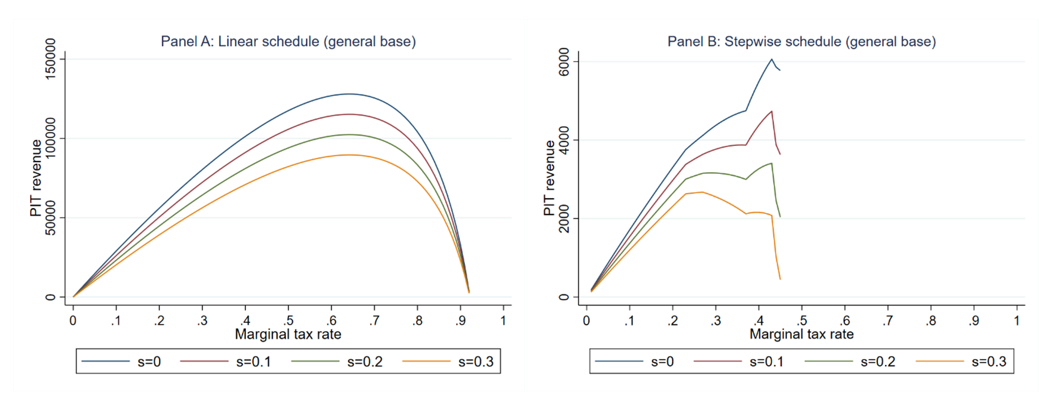
First, in most countries, the income tax has a stepwise schedule which influences the calculation of the actual revenue impact of a tax rate change and the characterisation of the Laffer Curve (see Figure 2). For instance, the Laffer Curves under a stepwise schedule are narrower than under a linear schedule. As a result, the revenue-maximising tax rates in a stepwise schedule are lower than in a linear schedule.
Figure 2 also shows that the smoothness of the curves in the linear schedule disappears in the stepwise schedule. The kinks detected in the stepwise schedule along the curves represent the discrete jump of marginal tax rates at bracket cut-offs.
Figure 2: Simulated Laffer Curves, linear schedule vs stepwise schedule
 (Click to enlarge)
Notes: Assuming taxpayers shift a fraction (s = 0, 0.1, 0.2, 0.3) of their non-savings or general income tax base towards the savings tax base.
Second, it is usual for tax reforms to entail simultaneous changes in more than one tax rate. However, most of the existing literature on the Laffer Curve ignores this by implicitly assuming a flat income tax structure, in other words, a tax with a single marginal tax rate.
This assumption has critical consequences for the profile of the Laffer Curve and the magnitude of the revenue-maximising tax rates.
Third, while the structural factors – linked to the design of the tax – have been examined in detail in the literature, only a few studies have analysed the implications of behavioural responses to taxation on the Laffer Curve. Our study adds to these studies by introducing the possibility of income shifting in a dual-income tax.
Whenever taxable incomes are subject to different marginal tax rates, the taxpayer is incentivised to move a fraction of high-marginal-rate bases to low-marginal-rate bases. Figure 2 illustrates how the presence of income shifting affects the magnitude of the revenue-maximising tax rate and, consequently, the profile of the Laffer Curve.
A key ingredient: the elasticity of taxable income
The total revenue impact of a tax rate change is composed of two opposing effects: mechanical and behavioural. While the former captures the tax revenue change without behavioural responses, the latter quantifies the revenue variation produced by behavioural changes.
Both mechanical and behavioural effects move in opposite directions and together allow the calculation of the actual revenue impact of a tax rate change and the characterisation of the Laffer Curve. The behavioural effect depends on a key parameter, the elasticity of taxable income. This behavioural elasticity captures all individuals’ responses to taxation – income shifting being one of them.
Our study estimates the ETI using the Instrumental Variables method considering the major changes in the Spanish personal income tax implemented during 2007-2016. We find that the ETI estimates are between 0.313 and 0.693 in the non-savings base and 0.708 and 0.823 in the savings base.
These estimates are especially high for women, single and separate tax filers in the general base, and for women, married and separate tax filers in the savings base. We find that the ETI estimates significantly affect the efficiency and revenue implications for tax policy.
An illustrative case study: the Spanish PIT
The computation of the individual revenue-maximising tax rates and elasticities requires complete knowledge of the taxpayers’ empirical distributions and tax bases in the personal income tax structure. This implies that it is necessary to have detailed tax microdata.
Using microdata from the Spanish Institute for Fiscal Studies, we calculate the total revenue impact of the 2012 tax reform, the revenue-maximising tax rate and the revenue-maximising elasticity of each taxpayer and its location on the Laffer Curve.
Applying the ETI estimates to the Spanish income tax demonstrates that 44.72% and 58.49% of the taxpaying population in the non-savings tax base and in the savings tax base were on the “normal” side of the Laffer Curve, respectively. On average, taxpayers in the non-savings base were 6.59 points above the maximum of the Laffer Curve, while taxpayers in the savings base were 24.73 points below it. This result indicates that the increase in the marginal tax rates in 2012 resulted in a revenue loss for half of the taxpaying population.
As a matter of fact, the fraction of total tax revenue lost through behavioural responses amounts to 53.77%. However, this fraction varies by population subgroup and decreases when we account for income-shifting responses, suggesting the presence of fiscal externalities in the Spanish PIT.
Our analysis shows that the Laffer Curve is not a fixed issue. Because its characterisation depends on a behavioural elasticity (the ETI), the Laffer Curve is exposed to behavioural factors such as avoidance channels and taxpayers’ circumstances.
These factors alter the shape of the Laffer Curve and the position of the taxpayers on it. These alterations have important policy implications in the study of the revenue capacity of tax systems, as they can lead to an over-/under-estimation of the magnitude of the revenue gain or loss associated with a change in the tax rates.


Recent Comments