Effective Marginal Tax Rates: Part 1

An Effective Marginal Tax Rate (EMTR) measures the loss resulting from income taxation combined with the withdrawal of a cash transfer or welfare benefit, applied to earning an extra (marginal) dollar of income. EMTRs are a result of the interaction of tax and welfare systems. Specifically, a high EMTR is a consequence of:

• progressive personal income tax rates
• means tested, i.e. tapered/phased out cash welfare benefits
• means tested in-kind benefits such as childcare assistance.

The EMTR applying for an individual or household resulting from a combination of income tax and withdrawal of particular welfare benefits can be presented in a chart that shows the EMTR at various points of earned income. Normally we look at the EMTR for the income unit in the tax or transfer system. In the income tax, the unit is the individual but in the welfare system it is often a couple or a couple with children, as this is the usual basis of assessment for social security purposes. This requires a range of assumptions about how the income is split within the couple; e.g. 100:0, 60:40 and so on. So the EMTR calculation implies that the marginal dollar of income is split in the same way, although we can also calculate on the basis that extra income goes to one or other in a couple, as shown later.

EMTR charts can be supplemented by disposable income graphs. If there were no tax-transfer system, these lines would be a ray through the origin. The tax-transfer system lifts the disposable income at the origin (when private income is zero) and flattens the disposable income line. Where EMTRs approach 100%, the disposable income line becomes completely flat, meaning that as private income rises disposable income is unchanged.

Figure 1 illustrates the EMTR for a couple that receives the age pension, as they earn increasing private income and the pension tapers as a result of the income test. It also shows the disposable income line for this couple. The line flattens over the range of the pension taper.

Figure 1: EMTR and disposable income (blue line) age pensioner couple

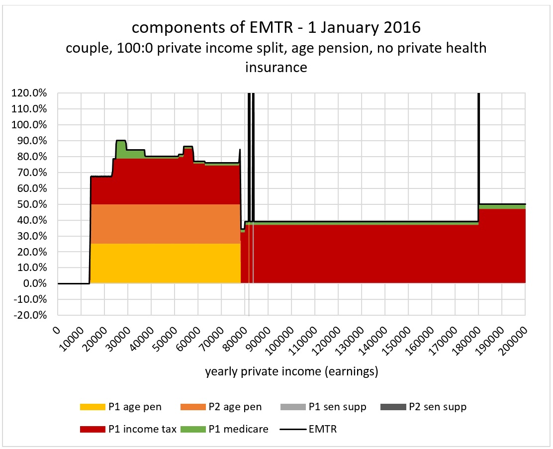
An EMTR chart can also show the importance of the different tax and welfare components in producing the EMTR at any point. Figure 2 shows how the different tax and welfare components contribute to the EMTR for the same age pensioner couple.

Figure 2: Components of EMTR for an age pensioner couple

High EMTRs arise from complex interactions of different payments and taxes and can only be unravelled by modellers using sophisticated computing. Because of this, it is tempting to suggest that they do not matter as individuals may have no idea what their EMTR is. The Productivity Commission rejected this argument, suggesting “If families are in a situation where they are facing a very high EMTR (especially if it exceeds 100%), most will be able to tell they are working for very little (or no) additional money” (p.887).

There have been studies of the number of people affected by high EMTRs – e.g. Harding 2008. (See also the brief survey in Ingles 2009).Typically such studies show relatively low numbers so impacted – in the range of 5-7% of working age Australians. However, not all those impacted will show up in these estimates as people may simply reduce their participation so as to bring their incomes below the levels where high EMTRs apply. Sole parents and to a lesser extent couples with children are the most likely family types to be affected, along with the unemployed. Harding notes that for mothers married to low income fathers, it may not be worth working because of benefit withdrawal and the cost of childcare.

EMTRs are necessarily a theoretical construct. The tax and welfare systems do not have exactly the same definition of ‘income’ (in some cases the latter includes assets and/or deeming) and moreover can apply over different time periods. In the case of say Newstart benefits, this period can be as little as a fortnight, as compared to annual income in the tax system. Nonetheless EMTRs are useful in analysing the disincentive effects of tax-transfer interactions, so long as we keep in mind that they are theoretical constructs.

Typically indirect taxes such as payroll tax and GST are not included in EMTR calculations. This partly reflects the lesser visibility of such taxes, and the possibility that there is a sort of fiscal illusion going on. Tax salience is important here. Macro calculations of ‘tax wedge’, by comparison, can take account of some indirect taxes. For example OECD calculations typically include payroll tax.

Participation tax rate

Instead of focusing on the EMTR for an extra dollar of private income, we can expand the unit of calculation for the EMTR. For example, we might look at the tax rate on an extra hour of earnings, or an extra day, or a whole week. These measures are in effect an Effective Average Tax Rate (EATR). The EATR is mathematically equal to the weighted average of the EMTRs over the relevant range.

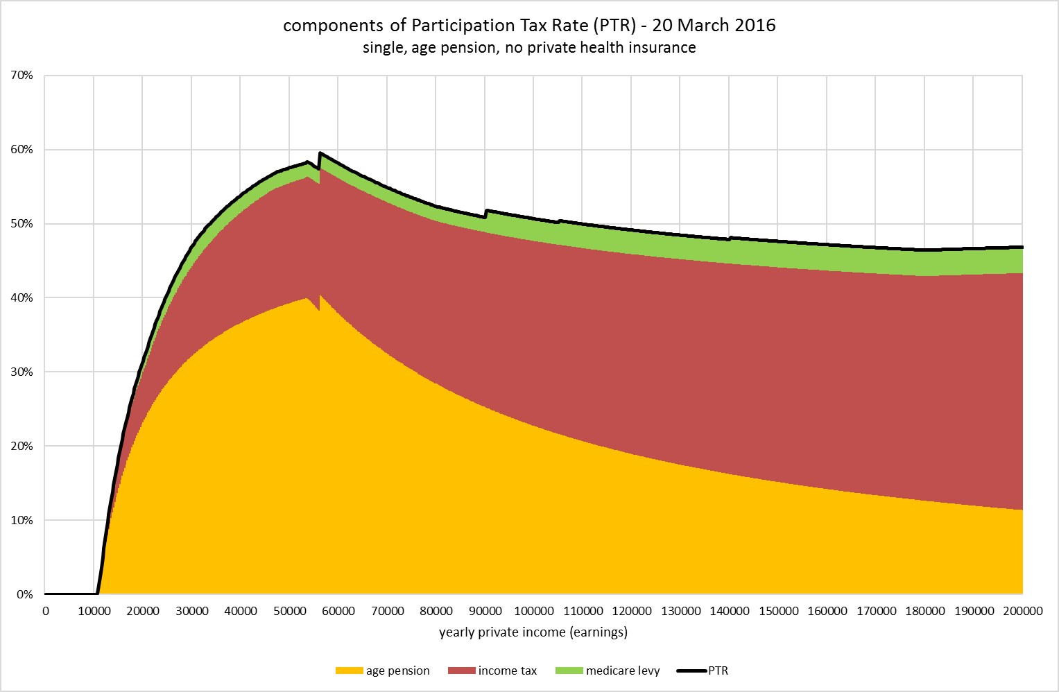
The concept can be expanded further to encompass the entirety of a person’s earnings. The resultant measure of the impact of the tax-transfer system on gains from taking up work is referred to as the Participation Tax Rate (PTR).  The PTR shows the net impost on working as a proportion of the gross salary. It is defined as 1 minus the financial gain to work as a proportion of gross earnings. It is essentially the average effective tax rate at the given income not including the value of benefits received, but taking account of benefit withdrawal.

Figure 3: Participation tax rate: Single age pensioner

Other welfare benefits including childcare

We also need to consider the range of programs which impact the EMTR. For example it has become more common to include childcare in these calculations.

The Productivity Commission Report on childcare found that the financial returns from a primary carer returning to work dropped off markedly over 5 days, for some earners becoming negative on the 4^th or 5^th day. A key question here is whether those returning to work are required by their employer to work a full week, or whether they have a choice to adjust their number of hours to work part-time or a shortened week. This Report noted that very high EMTRs result when a number of policies interact, in this case the welfare payments Family Tax Benefit (FTB) A and B, income tax rates and tapering of childcare assistance.

Modelling the impact of childcare assistance can be challenging. It requires assumptions about the number of hours of care which in turn relates to hours worked.With older school age children, childcare may not be necessary as they can stay at home for part of the day unattended. A little younger and outside school hours care comes into the picture. Younger still and we are probably talking about long day care.

There is also the added difficulty of relating childcare use to hourly rates of pay, especially where work is part-time. The usage pattern and hence costs will be different if hours worked are concentrated into a couple of days a week, as opposed to the same hours spread more or less evenly over a full week. Some people will also have access to informal assistance, for example from relatives.

Then, calculating the net impact as an EMTR raises the question of how much to increment childcare use with each increase in wages. An EMTR may require each plotted point to have a separate set of assumptions about childcare usage.

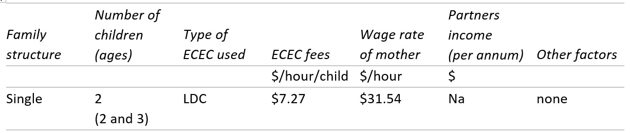
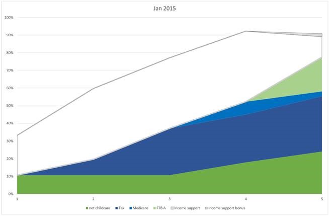
For example, if we model rising total income for a secondary earner (assuming the primary income is fixed), we know that income can rise either because hours are rising (implying more use of childcare) or because the implicit hourly wage rate is rising. To overcome this difficulty, such modelling tends to be based on ‘cameos’ – i.e. a stylised family type with an assumed income for the primary earner, and an assumed hourly wage rate for the secondary earner. Rising income of the latter corresponds with assumed changes in hours of care. This was the approach of the Productivity Commission, as shown in Figure 4. This figure relates to a single headed family, but the PC had 10 cameos in all with various family types.

Figure 4: Daily EMTR for sole parent (Productivity Commission)

Effective Marginal Tax Rates

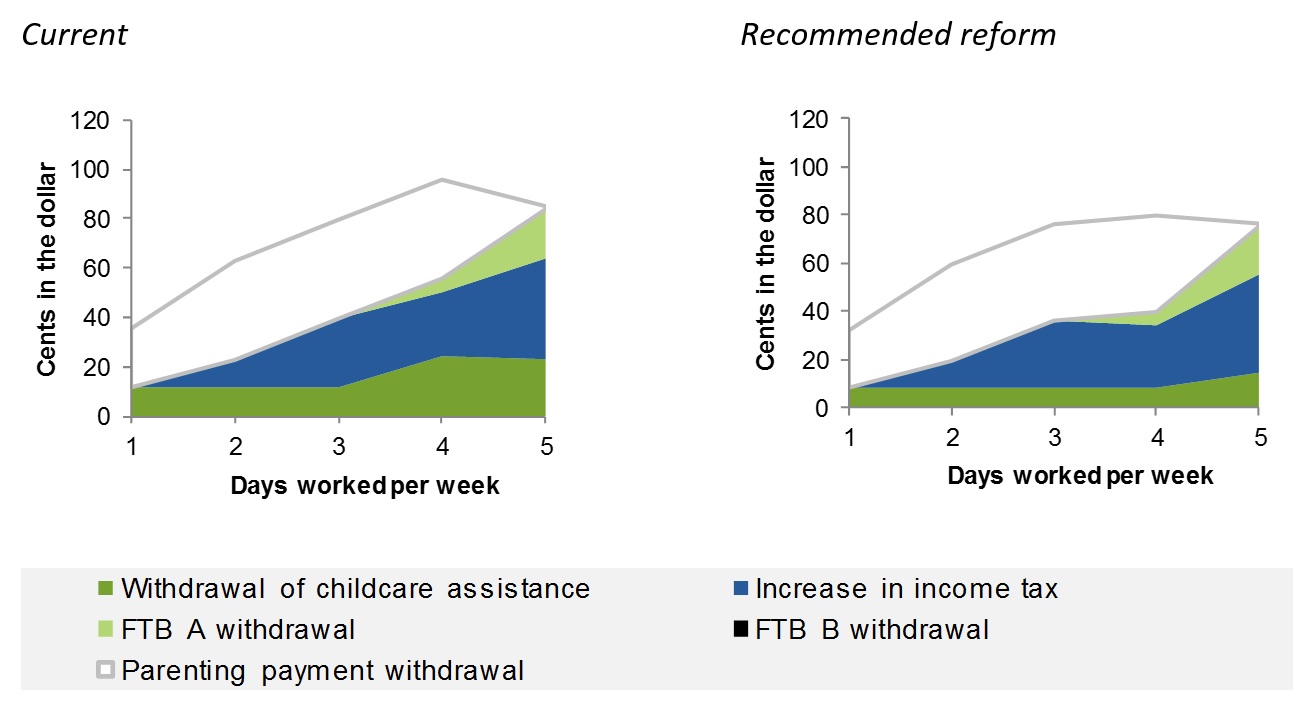
Source Productivity Commission 2015 Box E3 cameo 1. The ‘recommended reform’ is similar to the Government announced changes, although these changes have not been enacted.

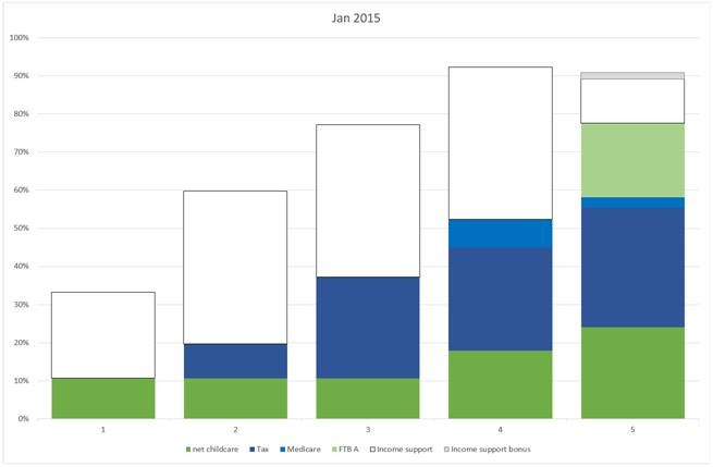
Figure 5: D Plunkett re-work of PC ‘Current’ chart

There are some minor differences in the results. There is still Parenting Payment (PPS) payable at day 4 of income, so the change to day 5 should show some percentage loss of PPS; however, the PC chart shows 0%. That has a flow on effect for FTB A as it’s not withdrawn while PPS is still in pay, consequently they show FTB A effects on day 4 whereas Figure 4 shows day 5 only. The PC labelling of withdrawal of childcare assistance is a misnomer, as it is actually increasing, not withdrawing. What they seem to be plotting is the change in net childcare costs. These caveats are here noted to make the point that EMTR modelling can be a complex and difficult task, and even experts may get different results.

The ‘area chart’ approach in the above chart tends to imply intermediate values that are not actually there. For something with discrete, and chunky, values like days worked, individual columns may be better, as shown in Figure 6.

Figure 6: EMTRs (daily) for sole parent as per PC cameo 1

Secondary earners in a couple

There is an argument that the high EMTR for a couple in a conventional EMTR chart is “felt” or directly impacts on the secondary or lower earner not the primary earner, if hours of the primary earner are fixed, or close to it. For example, if an income split of say 60:40 is assumed, this ratio is applied to the marginal dollar of each adult in the household to calculate the EMTR whereas in practice the marginal dollar will likely be earned by the secondary earner. We can model this using a fixed income for the primary earner.

Figure 7 EMTR chart if primary earner income is fixed, couple with 2 children age 2 & 3

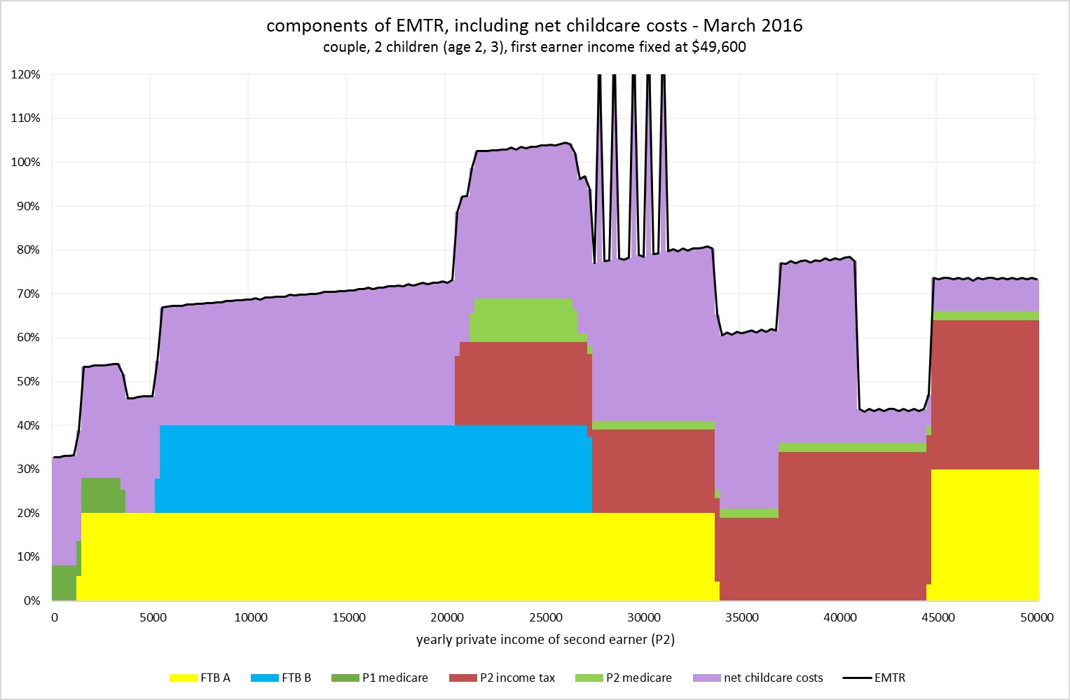
Note: Income of the primary earner is fixed at the minimum wage plus 41%, full year full time ($49600). Income of second earner is min wage plus 20% [1] ($20.75/hour). This ratio is based on the ratio of men’s to women’s wages, full time averages. Hours of care are 10/day at $8.50/hr. One aspect of long day care is that care is effectively charged for 10 hours in a full day, to a maximum of 50 hours per week. To mimic this, the assumption is that care hours grow faster than working hours, so that a 38 hour working week translates to 50 hours of care use.

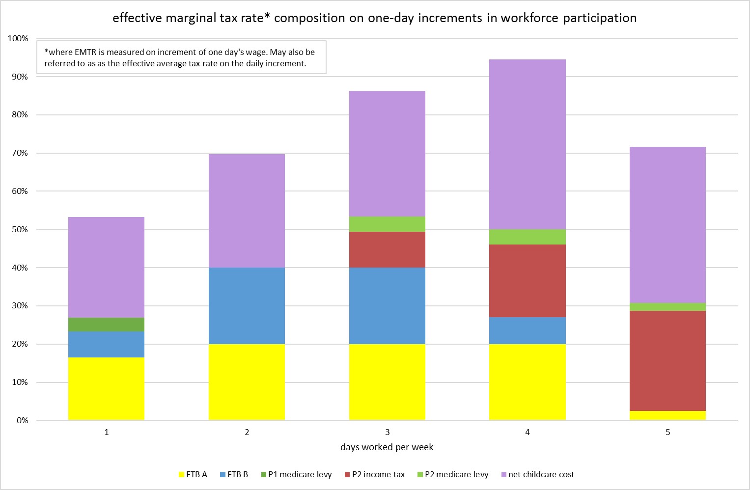
Figure 8 provides the same information in the more realistic bar chart, which recognises that childcare is typically charged in full-day blocks.

Figure 8 Per-day EMTR chart if primary earner income is fixed, couple with 2 children age 2 & 3

[1] We wished to use a graph for low wage but full time earners, not necessarily on the minimum wage. We had the idea of using parameters similar to the PC, but they have 10 different cameos with very wide ranges of assumed earnings.